One important procedure while formulating a mathematical model of a physical situation is scaling. Roughly speaking, scaling deals with choosing new, usually dimensionless variables and reformulate the problem expressed in these variables.
Example: Let t be the time. Every problem has a characteristic time tc, which is the smallest interval of time in which a notable change can be observed in the physical quantities. We then make the change of variables
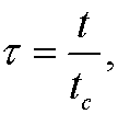
to achieve a dimensionless time ![]() .
.
Remark: We have different tc for different problems. If we study the motion of glaciers, tc can be of order years while tc can be of order microseconds if we for instance study nuclear reactions in atoms.
Example: (One dimensional heat conduction, see next part.) Consider a tall rod placed along the x-axis. The rod consists of a material with heat diffusivity k. We let u=u(x,t) denote the temperature in the point x at time t. The rod has the temperature 0 degrees at time t=0. We then keep the ends x=0 and x=l at the temperature T0 and examine how the temperature spreads in the rod. If the rod is long and slender, we can consider the problem one dimensional.

The temperature distribution is given by the one dimensional heat equation

We have the inital value

and the boundary conditions

As characteristic length lc we choose the length l of the rod and as characteristic temperature uc we choose the boundary temperature T0. As characteristic time tc we then choose l2/k, since k has the dimension [k]=L2/T. Thus we make the the change of variables

The chain rule now gives that
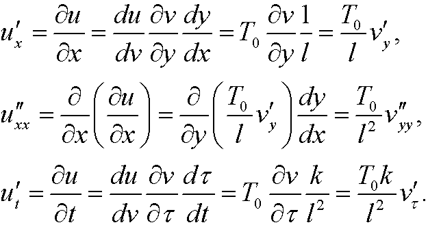
This implies that the heat equation is transformed to
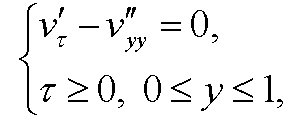
the initial value to
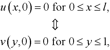
and the boundary conditions to
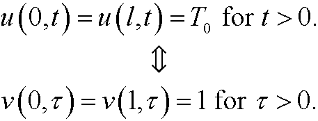
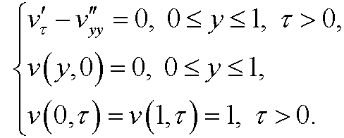
Alltogether, our transformed dimensionless boundary value problem will be
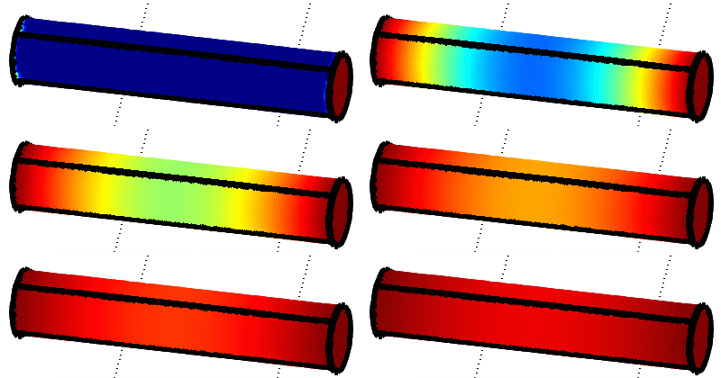
If we solve the problem we see that the heat will distribute in the rod as in the figure below.
Remark: If we changed the initial value

to

a natural choice of uc could be the mean value

However, it is more common and easier to choose
