In the most general case we will study systems of the type

where
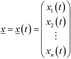
is an element in a vector space for every fix choice of t.
In this course we will mainly study systems on the form
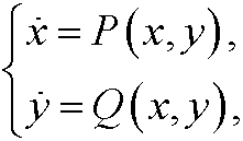
where x=x(t) and y=y(t) are regular real valued functions. In this case
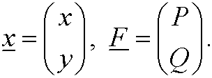
The solutions are defined on some interval
and can be drawn in the state space.
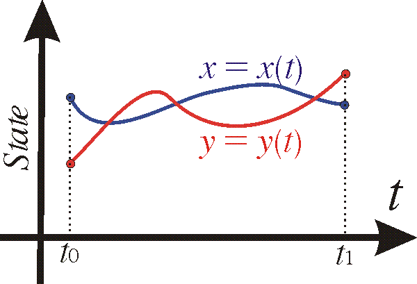
Alternatively they can be represented as a parametric curve in the xy-plane, also known as the phase plane.
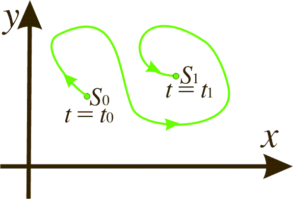
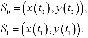
The arrows in the figure show how the system is developed in time. Here
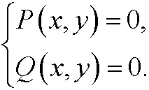
The equilibrium points are obtained by solving the system
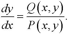
Since

we obtain
A phase portrait of the system is all orbits and equilibrium points in the phase plane. A quick way to get a phase portrait is to:
1) Find all equilibrium points by solving the system

2) Let a standard software (e.g. MATLAB) plot the solutions of

In part 9 we describe a more careful way to create phase portraits of linear dynamical systems, which we can get as approximations of general nonlinear systems by a first order taylor expansion. We give several concrete examples of continuous dynamical systems in the next part.